Neural Dynamics: A Primer (Hopfield Networks)
How does higher-order behavior emerge from billions of neurons firing?
This post is a basic introduction to thinking about the brain in the context of dynamical systems. I have found this way of thinking to be far more useful than the phrenology-like paradigms that pop science articles tend to love, in which spatially modular areas of the brain encode for specific functions. I tried to keep this introduction as simple and clear as possible, and accessible to anyone without background in neuroscience or mathematics.
For a list of seminal papers in neural dynamics, go here.
1. Emergent Behavior from Simple Parts
Physical systems made out of a large number of simple elements give rise to collective phenomena. For example, flying starlings:
Each starling follows simple rules: coordinating with seven neighbors, staying near a fixed point, and moving at a fixed speed. The result is emergent complex behavior of the flock.
The brain is similar: Each neuron follows a simple set of rules, and collectively, the neurons yield complex higher-order behavior, from keeping track of time to singing a tune. Granted, real neurons are highly varied and do not all follow the same set of rules, but we often assume that our model neurons do in order to keep things simple.
Although many types of these models exist, I will use Hopfield networks from this seminal paper to demonstrate some general properties. Hopfield networks were originally used to model human associative memory, in which a network of simple units converges into a stable state, in a process that I will describe below.
2. The Units of the Model
Following the paradigm described above, each neuron of the network abides by a simple set of rules. Each neuron is similar to a perceptron, a binary single neuron model. (There are some minor differences between perceptrons and Hopfield’s units, which have nondirectionality, direct stimulus input, and time constants, but I’ll not go into detail here.)
The inputs for each neuron are signals from the incoming neurons \([x_1.... x_n]\), which are multipled by the strengths of their connections \([w_1.... w_n]\), also called weights.

Once the signals and weights are multiplied together, the values are summed. If the total sum is greater than or equal to the threshold \(-b\), then the output value is \(1\), which means that the neuron fires. If the sum is less than the threshold, then the output is \(0\), which means that the neuron does not fire.
The rules above are modeled by the equation:
\[\begin{equation} f(x)= \begin{cases} 1,& \text{if}\ \sum_{k=1}^{n} w_k * x_k \geq -b\\ 0, & \text{otherwise} \end{cases} \end{equation}\]A Hopfield network consists of these neurons linked together without directionality. In hierarchical neural nets, the network has a directional flow of information (e.g. in Facebook’s facial recognition algorithm, the input is pixels and the output is the name of the person). However, in a Hopfield network, all of the units are linked to each other without an input and output layer. We consider the input to be the energy state of all the neurons before running the network, and the output to be the energy state after.
The strength of synaptic connectivity \(w_{ij}\) between neurons \(i\) and \(j\) follows the Hebbian learning rule, in which neurons that fire together wire together, and neurons that fire out of sync, fail to link:
\[w_{ij} = (2V_i - 1)(2V_j - 1)\]\(V_{i}\) and \(V_{j}\), the states of neurons \(i\) and \(j\), are either \(0\) (inactive) or \(1\) (active). As we can see by the equation, if both neurons are \(0\), or if both neurons are \(1\), then \(w_{ij} = 1\). If one neuron is \(0\), and the other is \(1\), then \(w_{ij} = -1\).
3. State Space
An important concept in Hopfield networks, and in dynamical systems more broadly, is state space, sometimes called the energy landscape.
The total Hopfield network has the value \(E\) associated with the total energy of the network, which is basically a sum of the activity of all the units. The network will tend towards lower energy states. We can think about this idea as represented by an energy landscape, seen below:
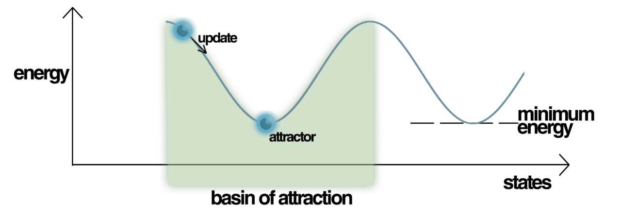
The y-axis represents the energy of the system \(E\), and the x-axis represents all the possible states that the system could be in. Out of all the possible energy states, the system will converge to a local minima, also called an attractor state, in which the energy of the total system is locally the lowest. Imagine a ball rolling around the hilly energy landscape, and getting caught in an attractor state.
While the above graph represents state space in one dimension, we can generalize the representation of state space to n dimensions.
4. Training and Running the Hopfield Network
Let’s walk through the Hopfield network in action, and how it could model human memory.
We initialize the network by setting the values of the neurons to a desired start pattern. The network runs according to the rules in the previous sections, with the value of each neuron changing depending on the values of its input neurons. Eventually, the network converges to an attractor state, the lowest energy value of the system.
Attractor states are “memories” that the network should “remember.” Before we initialize the network, we “train” it, a process by which we update the weights in order to set the memories as the attractor states. The network can therefore act as a content addressable (“associative”) memory system, which recovers memories based on similarity. If we train a four-neuron network so that state (-1, -1, -1, 1) is an attractor state, the network will converge to the attractor state given a starting state. For example, (-1, -1, -1, -1) will converge to (-1, -1, -1, 1).
So how do Hopfield networks relate to human memory?
Say you bite into a mint chocolate chip ice cream cone. That ice cream cone could be represented as a vector (-1, -1, -1, -1). Now say that for some reason, there is a deeply memorable mint chocolate chip ice cream cone from childhood– perhaps you were eating it with your parents and the memory has strong emotional saliency– represented by (-1, -1, -1, 1). As you bite into today’s ice cream cone, you find yourself thinking of the mint chocolate chip ice cream cone from years’ past. What happened? The starting point memory (-1, -1, -1, -1) converged to the system’s attractor state (-1, -1, -1, 1).

We can generalize this idea: some neuroscientists hypothesize that our perception of shades of color converges to an attractor state shade of that color. It’s also fun to think of Hopfield networks in the context of Proust’s famous madeleine passage, in which the narrator bites into a madeleine and is taken back to childhood. (His starting memory state of the madeleine converges to the attractor state of the childhood madeleine.)
As a caveat, as with most computational neuroscience models, we are operating on the 3rd level of Marr’s levels of analysis. In other words, we are not sure that the brain physically works like a Hopfield network. The brain could physically work like a Hopfield network, but the biological instantiation of memory is not the point; rather, we are seeking useful mathematical metaphors.
That concludes this basic primer on neural dynamics, in which we learned about emergence and state space. Other useful concepts include firing rate manifolds and oscillatory and chaotic behavior, which will be the content of a future post.
For a list of seminal papers in neural dynamics, go here.
I always appreciate feedback, so let me know what you think, either in the comments or through email.


Leave a comment